class: center, middle, inverse, title-slide # Logistic regression, LDA, QDA - Part 3 ### Dr. D’Agostino McGowan --- layout: true <div class="my-footer"> <span> Dr. Lucy D'Agostino McGowan <i>adapted from slides by Hastie & Tibshirani</i> </span> </div> --- ## Other forms of discriminant analysis `$$P(Y|X) = \frac{\pi_kf_k(x)}{\sum_{l=1}^K\pi_lf_l(x)}$$` -- * When `\(f_k(x)\)` are **normal** densities with the **same covariance** matrix `\(\mathbf\Sigma\)` in each class, this is **linear discriminant analysis** -- * When `\(f_k(x)\)` are **normal** densities with **different covariance** matrices `\(\mathbf\Sigma_k\)` in each class, this is **quadratic discriminant analysis** -- * Lots of other forms are possible! --- ## Quadratic Discriminant Analysis <img src = "img/05/qda.png" height = 250></img> `$$\delta_k(x) = -\frac{1}{2}(x-\mu_k)^T\mathbf\Sigma_k^{-1}(x-\mu_k)+\log\pi_k$$` .question[ Why do you think this is called **quadratic** discriminant analysis? ] -- * Because the `\(\mathbf\Sigma_k\)` are different, the quadratic terms matter --- ## Let's see it in R .small[ ```r library(MASS) *model <- qda(default ~ balance + student, data = Default) predictions <- predict(model) ``` ] * Use the `qda()` function in R from the **MASS** package --- ## Let's see it in R * Let's use LDA to visualize the data .small[ ```r *model <- lda(Species ~ ., data = iris) predictions <- predict(model) ``` ] --- ## Let's see it in R * Let's use LDA to visualize the data .small[ ```r model <- lda(Species ~ ., data = iris) predictions <- predict(model) *plot_data <- data.frame(outcome = iris$Species, * lda = predictions$x) head(plot_data) ``` ``` ## outcome lda.LD1 lda.LD2 ## 1 setosa 8.061800 0.3004206 ## 2 setosa 7.128688 -0.7866604 ## 3 setosa 7.489828 -0.2653845 ## 4 setosa 6.813201 -0.6706311 ## 5 setosa 8.132309 0.5144625 ## 6 setosa 7.701947 1.4617210 ``` ] --- ## Let's see it in R * Let's use LDA to visualize the data .small[ ```r *ggplot(data = plot_data, * mapping = aes(x = lda.LD1, y = lda.LD2, color = outcome)) + * geom_point() ``` 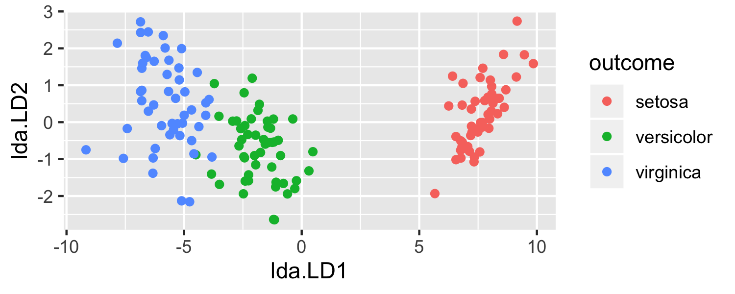<!-- --> ] --- ## ggplot2 `\(\in\)` tidyverse .pull-left[  ] .pull-right[ - **ggplot2** is tidyverse's data visualization package - The `gg` in "ggplot2" stands for Grammar of Graphics - It is inspired by the book **Grammar of Graphics** by Leland Wilkinson ^† - A grammar of graphics is a tool that enables us to concisely describe the components of a graphic 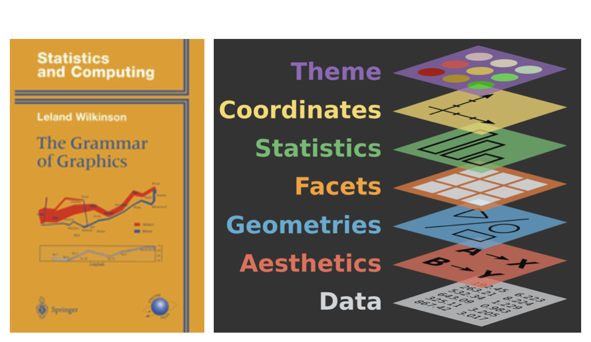 ] .footnote[ ^† Source: [BloggoType](http://bloggotype.blogspot.com/2016/08/holiday-notes2-grammar-of-graphics.html) ] --- ## ggplot2 .question[ What function creates the plot? ] .small[ ```r ggplot(data = plot_data, mapping = aes(x = lda.LD1, y = lda.LD2, color = outcome)) + geom_point() + labs(x = "LD1", y = "LD2") ``` <!-- --> ] --- ## ggplot2 .question[ What data set is being plotted? ] .small[ ```r ggplot(data = plot_data, mapping = aes(x = lda.LD1, y = lda.LD2, color = outcome)) + geom_point() + labs(x = "LD1", y = "LD2") ``` <!-- --> ] --- ## ggplot2 .question[ Which variables are on the x- and y-axis? ] .small[ ```r ggplot(data = plot_data, mapping = aes(x = lda.LD1, y = lda.LD2, color = outcome)) + geom_point() + labs(x = "LD1", y = "LD2") ``` 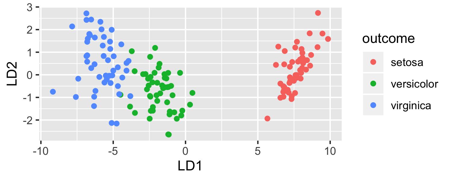<!-- --> ] --- ## ggplot2 .question[ What variable in the dataset determines the color? ] .small[ ```r ggplot(data = plot_data, mapping = aes(x = lda.LD1, y = lda.LD2, color = outcome)) + geom_point() + labs(x = "LD1", y = "LD2") ``` <!-- --> ] --- ## ggplot2 .question[ What does `geom_point()` mean? ] .small[ ```r ggplot(data = plot_data, mapping = aes(x = lda.LD1, y = lda.LD2, color = outcome)) + geom_point() + labs(x = "LD1", y = "LD2") ``` <!-- --> ] --- ## Hello ggplot2! - `ggplot()` is the main function in ggplot2 and plots are constructed in layers - The structure of the code for plots can often be summarized as ```r ggplot + geom_xxx ``` -- or, more precisely .small[ ```r ggplot(data = [dataset], mapping = aes(x = [x-variable], y = [y-variable])) + geom_xxx() + other options ``` ] --- ## Hello ggplot2! - To use ggplot2 functions, first load tidyverse -- - For help with the ggplot2, see [ggplot2.tidyverse.org](http://ggplot2.tidyverse.org/) --- <!-- --> * What is going on here? -- * LDA is projecting the samples `\(X\)` onto a _hyperplane_ with `\(K-1\)` dimensions. -- .question[ What is K here? ] --- <!-- --> * What is going on here? * LDA is projecting the samples `\(X\)` onto a _hyperplane_ with `\(K-1\)` dimensions. * Why does this work? * LDA essentially classifies to the closest centroid, and they span a K - 1 dimensional plane. -- * Even when K > 3, we can find the "best" 2-dimensional plane for vizualizing the discriminant rule by using the first two discriminant variables (LD1 and LD2) --- ## Logistic Regression versus LDA * For the two-class problem ( `\(K=2\)` ), LDA takes the form `$$\log\left(\frac{p_1(x)}{1-p_1(x)}\right)=\log\left(\frac{p_1}{p_2}\right) = c_0 + c_1x_1 + \dots+ c_px_p$$` -- * This is the same form as logistic regression -- * The difference is in how the parameters are estimated -- * Logistic regression uses the conditional likelihood based on `\(P(Y|X)\)` (**discriminative learning**) -- * LDA uses the full likelihood based on `\(P(X,Y)\)` (**generative learning**) -- * The results are often similar --- ## Summary * Logistic regression is very popular for classification, especially when `\(K = 2\)` * LDA is useful when `\(n\)` is small, or the classes are well separated, and normality assumptions are reasonable. Also when `\(K > 2\)` -- * QDA is _similar_ to LDA, but it is more flexible because it allows the covariance of the predictors to be different for each class, `\(k\)` -- * See Section 4.5 in your book for some comparisons of logistic regression, LDA, and KNN.