class: center, middle, inverse, title-slide # Cross validation ### Dr. D’Agostino McGowan --- layout: true <div class="my-footer"> <span> Dr. Lucy D'Agostino McGowan <i>adapted from slides by Hastie & Tibshirani</i> </span> </div> --- ## <i class="fas fa-laptop"></i> `CV` - Go to the [sta-363-s20 GitHub organization](https://github.com/sta-363-s20) and search for `appex-03-cv` - Clone this repository into RStudio Cloud --- ## Cross validation ### 💡 Big idea * We have determined that it is sensible to use a _test_ set to calculate metrics like prediction error -- .question[ Why? ] --- ## Cross validation ### 💡 Big idea * We have determined that it is sensible to use a _test_ set to calculate metrics like prediction error .question[ How have we done this so far? ] --- ## Cross validation ### 💡 Big idea * We have determined that it is sensible to use a _test_ set to calculate metrics like prediction error * What if we don't have a seperate data set to test our model on? -- * 🎉 We can use **resampling** methods to **estimate** the test-set prediction error --- ## Training error versus test error .question[ What is the difference? Which is typically larger? ] -- * The **training error** is calculated by using the same observations used to fit the statistical learning model -- * The **test error** is calculated by using a statistical learning method to predict the response of **new** observations -- * The **training error rate** typically _underestimates_ the true prediction error rate --- 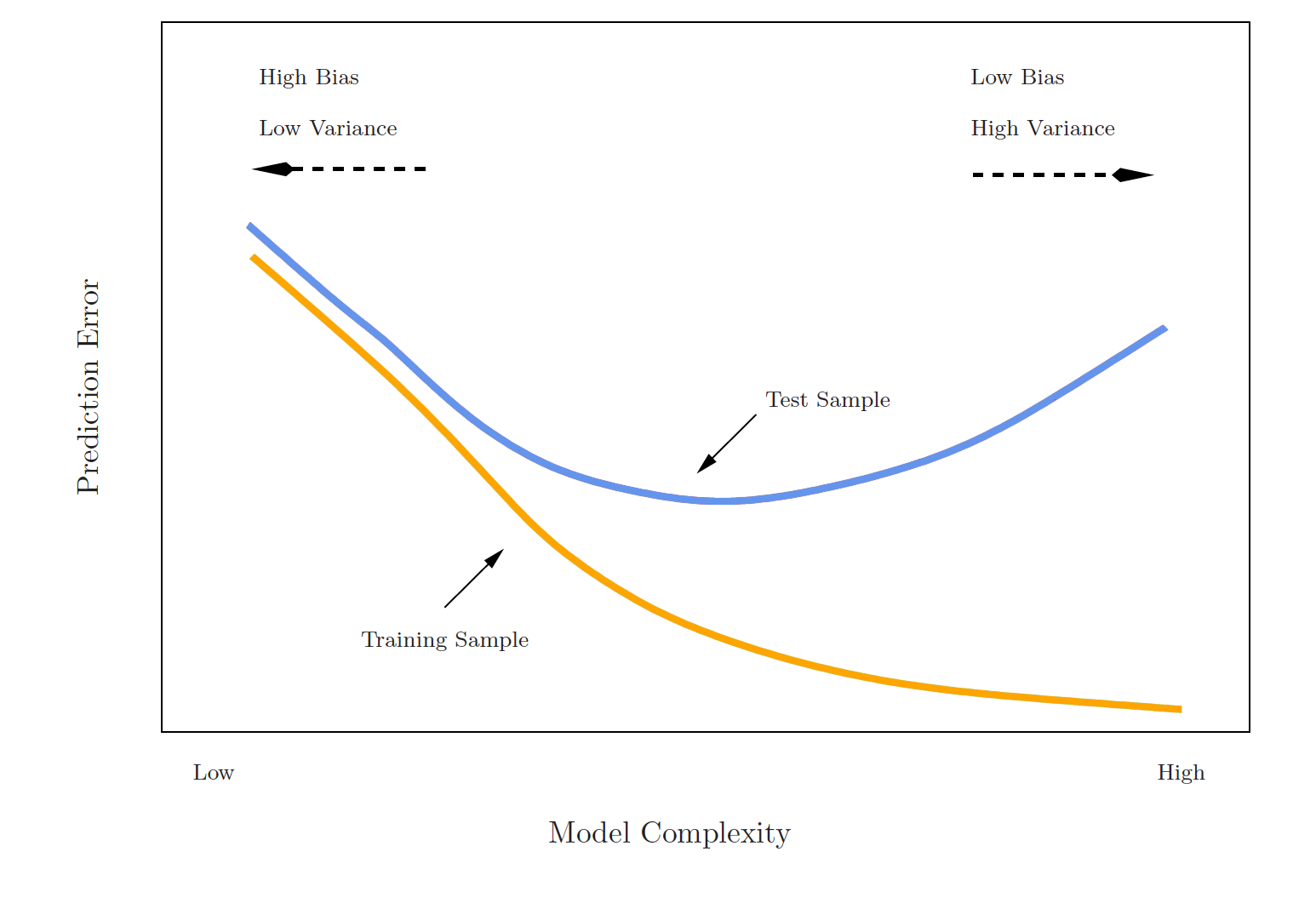 --- ## Estimating prediction error * Best case scenario: We have a large data set to test our model on -- * This is not always the case! -- 💡 Let's instead find a way to estimate the test error by holding out a subset of the training observations from the model fitting process, and then applying the statistical learning method to those held out observations --- ## Approach #1: Validation set * Randomly divide the available set up samples into two parts: a **training set** and a **validation set** -- * Fit the model on the **training set**, calculate the prediction error on the **validation set** -- .question[ If we have a **quantitative predictor** what metric would we use to calculate this test error? ] -- * Often we use Mean Squared Error (MSE) --- ## Approach #1: Validation set * Randomly divide the available set up samples into two parts: a **training set** and a **validation set** * Fit the model on the **training set**, calculate the prediction error on the **validation set** .question[ If we have a **qualitative predictor** (classification) what metric would we use to calculate this test error? ] -- * Often we use misclassification rate --- ## Approach #1: Validation set Auto example: * We have 392 observations * Trying to predict `mpg` from `horsepower` * We can split the data in half and use 196 to fit the model and 196 to test 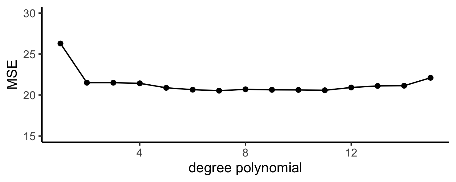<!-- --> --- ## Approach #1: Validation set Auto example: * We have 392 observations * Trying to predict `mpg` from `horsepower` * We can split the data in half and use 196 to fit the model and 196 to test - **what if we did this many times?** 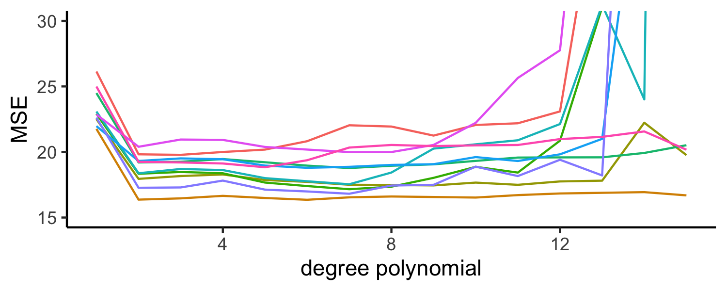<!-- --> --- ## Approach #1: Validation set (Drawbacks) * the validation estimate of the test error can be highly variable, depending on which observations are included in the training set and which observations are included in the validation set -- * In the validation approach, only a subset of the observations (those that are included in the training set rather than in the validation set) are used to fit the model -- * Therefore, the validation set error may tend to **overestimate** the test error for the model fit on the entire data set --- ## Approach #2: K-fold cross validation 💡 The idea is to do the following: * Randomly divide the data into `\(K\)` equal-sized parts -- * Leave out part `\(k\)`, fit the model to the other `\(K - 1\)` parts (combined) -- * Obtain predictions for the left-out `\(k\)`th part -- * Do this for each part `\(k = 1, 2,\dots K\)`, and then combine the results --- ## Let's do it in R! .small[ ```r sample(1:nrow(Auto)) ``` ``` ## [1] 266 72 207 312 122 268 299 101 261 380 211 355 79 88 183 174 295 1 ## [19] 281 310 118 265 94 115 257 156 313 196 200 307 137 60 69 308 121 277 ## [37] 25 86 381 362 363 340 304 153 67 29 202 356 182 162 17 203 270 204 ## [55] 10 134 36 9 374 109 98 273 353 4 18 239 24 23 390 337 139 26 ## [73] 89 254 347 379 44 209 359 348 117 37 242 21 373 39 238 111 188 278 ## [91] 32 216 47 383 231 177 318 300 324 386 87 164 385 288 62 170 389 154 ## [109] 230 329 191 248 369 250 225 15 263 138 330 55 186 149 165 83 316 227 ## [127] 48 367 368 141 213 287 201 335 145 31 176 234 143 146 131 166 148 20 ## [145] 352 244 247 73 193 167 332 96 262 197 64 43 226 327 82 235 3 50 ## [163] 382 12 199 271 298 232 328 172 8 223 292 221 222 80 45 208 358 370 ## [181] 171 35 387 245 240 22 124 309 365 372 284 105 11 311 7 255 140 354 ## [199] 93 74 150 184 85 53 123 142 110 68 215 27 49 302 343 290 61 51 ## [217] 132 99 175 272 251 256 130 321 289 349 269 5 246 351 303 276 243 187 ## [235] 136 249 346 107 100 14 91 319 157 293 275 65 59 54 219 16 282 113 ## [253] 325 70 192 95 66 296 97 301 322 78 377 6 81 294 90 34 338 317 ## [271] 92 205 169 342 38 252 258 120 129 241 52 163 228 334 280 339 264 181 ## [289] 194 267 364 77 42 127 375 180 345 214 135 190 220 133 151 119 320 210 ## [307] 198 185 392 128 391 58 206 13 378 179 212 41 19 104 331 147 46 2 ## [325] 195 306 253 30 297 103 279 33 102 260 274 71 152 161 126 236 360 388 ## [343] 155 106 341 160 114 75 224 178 305 376 384 63 350 357 366 116 217 40 ## [361] 218 108 233 336 371 112 229 84 314 168 323 237 28 326 315 56 286 76 ## [379] 285 125 57 344 283 259 173 159 158 333 361 144 189 291 ``` ] --- ## Let's do it in R! .question[ What is this code doing? ] .small[ ```r sample(1:nrow(Auto)) ``` ``` ## [1] 146 341 313 69 64 366 172 31 379 7 190 163 145 280 106 248 294 271 ## [19] 368 203 246 103 147 207 361 355 80 144 318 252 122 250 56 320 319 50 ## [37] 13 127 135 218 179 119 116 201 18 140 91 59 21 19 333 375 11 185 ## [55] 6 262 255 4 274 286 141 210 138 107 363 231 300 199 343 238 292 226 ## [73] 339 181 117 177 284 86 260 212 281 93 120 384 241 167 189 283 92 111 ## [91] 291 367 170 240 143 259 208 38 192 235 71 328 139 96 287 353 354 74 ## [109] 109 85 217 121 184 68 83 258 39 133 220 304 149 14 359 142 104 345 ## [127] 391 90 347 95 314 356 324 176 42 150 24 168 346 60 327 8 110 243 ## [145] 99 228 25 79 129 348 206 102 323 115 216 5 46 254 72 124 169 221 ## [163] 239 385 290 321 22 202 76 378 40 78 276 365 52 195 285 325 329 362 ## [181] 157 236 65 358 41 317 196 57 386 30 153 265 376 301 33 81 193 29 ## [199] 173 295 310 152 264 298 377 118 305 47 340 387 332 256 178 392 175 383 ## [217] 100 322 183 70 188 45 272 336 390 165 374 357 306 166 174 308 303 214 ## [235] 382 108 156 334 299 3 155 307 101 112 51 277 232 293 273 229 244 278 ## [253] 209 263 16 73 269 344 245 364 158 62 337 261 242 32 219 279 128 372 ## [271] 326 335 234 249 389 54 58 61 44 105 49 28 97 20 10 26 126 88 ## [289] 233 316 134 171 48 98 9 352 131 130 123 373 197 237 247 148 312 2 ## [307] 17 282 132 330 315 349 198 187 227 350 159 137 270 289 204 222 55 351 ## [325] 34 180 215 67 87 94 84 380 161 211 154 12 288 338 213 160 369 253 ## [343] 309 296 23 182 360 331 225 27 162 75 302 82 53 370 230 205 136 200 ## [361] 113 223 267 191 186 43 194 311 66 164 114 381 388 89 275 125 77 35 ## [379] 297 251 371 15 1 257 266 36 37 342 224 268 63 151 ``` ] --- ## Let's do it in R! .small[ ```r K <- 5 Auto <- Auto %>% * slice(sample(1:nrow(Auto))) %>% mutate(k = rep(1:K, length.out = nrow(Auto))) ``` ] --- ## Let's do it in R! .small[ ```r K <- 5 Auto <- Auto %>% * slice(sample(1:nrow(Auto))) %>% * mutate(k = rep(1:K, length.out = nrow(Auto))) ``` ] --- ## Let's do it in R! .small[ ```r K <- 5 Auto <- Auto %>% slice(sample(1:nrow(Auto))) %>% mutate(k = rep(1:K, length.out = nrow(Auto))) Auto %>% group_by(k) %>% summarise(n = n()) ``` ``` ## # A tibble: 5 x 2 ## k n ## <int> <int> ## 1 1 79 ## 2 2 79 ## 3 3 78 ## 4 4 78 ## 5 5 78 ``` ] --- ## Estimating prediction error (quantitative outcome) * Split the data into K parts, where `\(C_1, C_2, \dots, C_k\)` indicate the indices of observations in part `\(k\)` `$$CV_{(K)} = \sum_{k=1}^K\frac{n_k}{n}MSE_k$$` -- * `\(MSE_k = \sum_{i \in C_k} (y_i - \hat{y}_i)^2/n_k\)` -- * `\(n_k\)` is the number of observations in group `\(k\)` * `\(\hat{y}_i\)` is the fit for observation `\(i\)` obtained from the data with the part `\(k\)` removed -- * If we set `\(K = n\)`, we'd have `\(n-fold\)` cross validation which is the same as **leave-one-out cross validation** (LOOCV) --- ## Let's see it in R! .question[ What pieces of the equation have a _k_ in them? ] -- ```r Auto1 <- Auto %>% filter(k != 1) model1 <- lm(mpg ~ horsepower, data = Auto1) Auto %>% filter(k == 1) %>% mutate(p = predict(model1, newdata = .)) %>% summarise(mse_1 = mean((mpg - p)^2), n_1 = n()) ``` ``` ## mse_1 n_1 ## 1 23.02586 79 ``` --- ## Let's see it in R! ```r *Auto1 <- Auto %>% * filter(k != 1) model1 <- lm(mpg ~ horsepower, data = Auto1) Auto %>% filter(k == 1) %>% mutate(p = predict(model1, newdata = .)) %>% summarise(mse_1 = mean((mpg - p)^2), n_1 = n()) ``` ``` ## mse_1 n_1 ## 1 23.02586 79 ``` --- ## Let's see it in R! ```r Auto1 <- Auto %>% filter(k != 1) *model1 <- lm(mpg ~ horsepower, data = Auto1) Auto %>% filter(k == 1) %>% mutate(p = predict(model1, newdata = .)) %>% summarise(mse_1 = mean((mpg - p)^2), n_1 = n()) ``` ``` ## mse_1 n_1 ## 1 23.02586 79 ``` --- ## Let's see it in R! ```r Auto1 <- Auto %>% filter(k != 1) model1 <- lm(mpg ~ horsepower, data = Auto1) *Auto %>% * filter(k == 1) %>% mutate(p = predict(model1, newdata = .)) %>% summarise(mse_1 = mean((mpg - p)^2), n_1 = n()) ``` ``` ## mse_1 n_1 ## 1 23.02586 79 ``` --- ## Let's see it in R! ```r Auto1 <- Auto %>% filter(k != 1) model1 <- lm(mpg ~ horsepower, data = Auto1) Auto %>% filter(k == 1) %>% * mutate(p = predict(model1, newdata = .)) %>% summarise(mse_1 = mean((mpg - p)^2), n_1 = n()) ``` ``` ## mse_1 n_1 ## 1 23.02586 79 ``` --- ## Let's see it in R! ```r Auto1 <- Auto %>% filter(k != 1) model1 <- lm(mpg ~ horsepower, data = Auto1) Auto %>% filter(k == 1) %>% mutate(p = predict(model1, newdata = .)) %>% * summarise(mse_1 = mean((mpg - p)^2), * n_1 = n()) ``` ``` ## mse_1 n_1 ## 1 23.02586 79 ``` --- ## Let's see it in R! ```r Auto1 <- Auto %>% filter(k != 1) model1 <- lm(mpg ~ horsepower, data = Auto1) Auto %>% filter(k == 1) %>% mutate(p = predict(model1, newdata = .)) %>% summarise(mse_1 = mean((mpg - p)^2), n_1 = n()) ``` ``` ## mse_1 n_1 ## 1 23.02586 79 ``` * Now we just have to do this 4 more times! -- 😅 --- class: center, middle ## 👍 If you have to copy/paste code more than 3 times, write a function! --- ## Let's see it in R! ```r *mse_k <- function(K = 1) { Auto_k <- Auto %>% filter(k != K) model_k <- lm(mpg ~ horsepower, data = Auto_k) Auto %>% filter(k == K) %>% mutate(p = predict(model_k, newdata = .)) %>% summarise(mse_k = mean((mpg - p)^2), n_k = n()) *} ``` --- ## Let's see it in R! ```r mse_k <- function(K = 1) { Auto_k <- Auto %>% * filter(k != K) model_k <- lm(mpg ~ horsepower, data = Auto_k) Auto %>% * filter(k == K) %>% mutate(p = predict(model_k, newdata = .)) %>% summarise(mse_k = mean((mpg - p)^2), n_k = n()) } ``` --- ## Let's see it in R! ```r mse_k() ``` ``` ## mse_k n_k ## 1 23.02586 79 ``` --- ## Let's see it in R! ```r mse_k(K = 1) ``` ``` ## mse_k n_k ## 1 23.02586 79 ``` --- ## Let's see it in R! ```r mse_k(K = 1) ``` ``` ## mse_k n_k ## 1 23.02586 79 ``` ```r mse_k(K = 2) ``` ``` ## mse_k n_k ## 1 30.922 79 ``` ```r mse_k(K = 3) ``` ``` ## mse_k n_k ## 1 19.48487 78 ``` -- * Uh-oh we are copy/pasting again! --- ## purrr `\(\in\)` tidyverse .pull-left[  ] .pull-right[ - **purrr** is a package for _iterating_ in R - The functions we will use are all `map_xxx()` functions ] --- ## `map(.x, .f, ...)` -- ### for every element of `.x` do `.f` --- ## Example .small[ ```r map(1:5, ~ .x * 2) ``` ``` ## [[1]] ## [1] 2 ## ## [[2]] ## [1] 4 ## ## [[3]] ## [1] 6 ## ## [[4]] ## [1] 8 ## ## [[5]] ## [1] 10 ``` ] -- * By default, the output will be a **list** -- * You can dictate your desired output type by specifying `map_xxx()` for example to output a numeric (double) vector, use `map_dbl()` --- ## Example .small[ ```r map_dbl(1:5, ~ .x * 2) ``` ``` ## [1] 2 4 6 8 10 ``` ] --- ## `map_xxx(.x, .f)` * `map()`: list * `map_dbl()`: double * `map_int()` * `map_lgl()` * `map_chr()` * `map_df()` -- .question[ What do you think the rest of these output? ] --- ## `map_xxx(.x, .f)` * `map()`: list * `map_dbl()`: double * `map_int()`: integer * `map_lgl()`: logical * `map_chr()`: character * `map_df()`: data frame .question[ What do you think the rest of these output? ] --- ## Back to our example! .pull-left[ .small[ ```r map(1:K, ~ mse_k(.x)) ``` ``` ## [[1]] ## mse_k n_k ## 1 23.02586 79 ## ## [[2]] ## mse_k n_k ## 1 30.922 79 ## ## [[3]] ## mse_k n_k ## 1 19.48487 78 ## ## [[4]] ## mse_k n_k ## 1 19.9612 78 ## ## [[5]] ## mse_k n_k ## 1 26.69468 78 ``` ] ] .pull-right[ .question[ How can I get these into a data frame? ] ] --- ## Let's see it in R! .small[ ```r map_df(1:K, ~ mse_k(.x)) ``` ``` ## mse_k n_k ## 1 23.02586 79 ## 2 30.92200 79 ## 3 19.48487 78 ## 4 19.96120 78 ## 5 26.69468 78 ``` ] -- .question[ What do I need to do with these to estimate the prediction error? ] .small[ ```r map_df(1:K, ~ mse_k(.x)) %>% summarise(cv_5 = sum(n_k / sum(n_k) * mse_k)) ``` ``` ## cv_5 ## 1 24.03281 ``` ] --- ## Special Case! * With _linear_ regression, you can actually calculate the LOOCV error without having to iterate! `$$CV_{(n)} = \frac{1}{n}\sum_{i=1}^n\left(\frac{y_i-\hat{y}_i}{1-h_i}\right)^2$$` -- * `\(\hat{y}_i\)` is the `\(i\)`th fitted value from the linear model -- * `\(h_i\)` is the diagonal of the "hat" matrix (remember that! 🎓) --- ## Picking `\(K\)` * `\(K\)` can vary from 2 (splitting the data in half each time) to `\(n\)` (LOOCV) -- * LOOCV is sometimes useful but usually the estimates from each fold are very correlated, so their average can have a **high variance** -- * A better choice tends to be `\(K=5\)` or `\(K=10\)` --- ## Bias variance trade-off * Since each training set is only `\((K - 1)/K\)` as big as the original training set, the estimates of prediction error will typically be **biased** upward -- * This bias is minimized when `\(K = n\)` (LOOCV), but this estimate has a **high variance** -- * `\(K =5\)` or `\(K=10\)` provides a nice compromise for the bias-variance trade-off --- ## Approach #2: K-fold Cross Validation Auto example: * We have 392 observations * Trying to predict `mpg` from `horsepower` 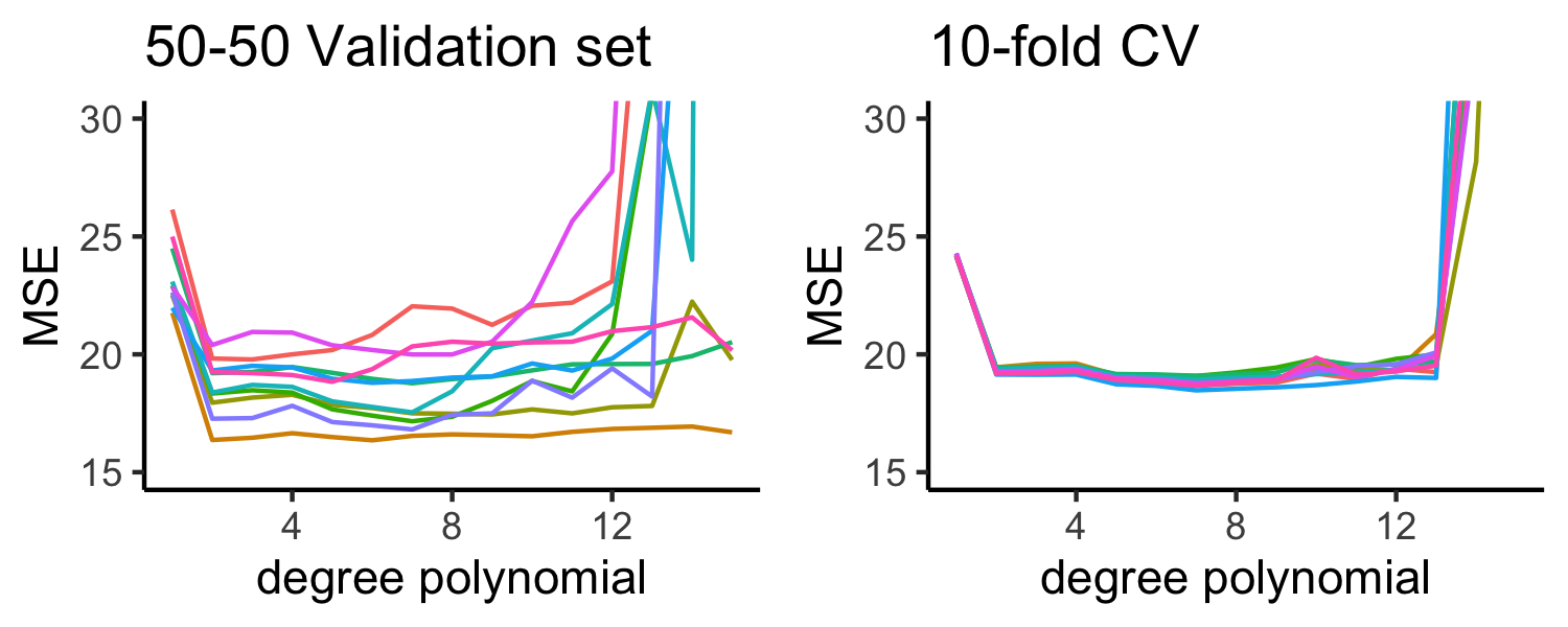<!-- --> --- ## Estimating prediction error (qualitative outcome) * The premise is the same as cross valiation for quantitative outcomes * Split the data into K parts, where `\(C_1, C_2, \dots, C_k\)` indicate the indices of observations in part `\(k\)` `$$CV_K = \sum_{k=1}^K\frac{n_k}{n}Err_k$$` -- * `\(Err_k = \sum_{i\in C_k}I(y_i\neq\hat{y}_i)/n_k\)` (missclassification rate) -- * `\(n_k\)` is the number of observations in group `\(k\)` * `\(\hat{y}_i\)` is the fit for observation `\(i\)` obtained from the data with the part `\(k\)` removed --- ## <i class="fas fa-laptop"></i> `CV` - Go to the [sta-363-s20 GitHub organization](https://github.com/sta-363-s20) and search for `appex-03-cv` - Clone this repository into RStudio Cloud - Complete the exercises - Remember to **knit, commit, push!**