tidymodels

tidymodelsDr. D’Agostino McGowan1 / 48

`tidymodels`

Go to the sta-363-s20 GitHub organization and search for appex-04-tidymodels
Go to RStudio Pro
rstudio.hpc.ar53.wfu.edu:8787
pw: R2D2Star!

2 / 48

tidymodels

tidyverse.org

tidymodels is an opinionated collection of R packages designed for modeling and statistical analysis.
All packages share an underlying philosophy and a common grammar.

3 / 48

Dr. Lucy D'Agostino McGowan  adapted from Alison Hill's Introduction to ML with the Tidyverse

Step 1: Specify the modelPick the model
4 / 48

Dr. Lucy D'Agostino McGowan  adapted from Alison Hill's Introduction to ML with the Tidyverse

Step 1: Specify the modelPick the model
Set the engine
4 / 48

Specify the model

linear_reg() %>%
  set_engine("lm")

5 / 48

Specify the model

linear_reg() %>%
  set_engine("glmnet")

6 / 48

Specify the model

linear_reg() %>%
  set_engine("spark")

7 / 48

Specify the model

decision_tree() %>%
  set_engine("ranger")

8 / 48

Specify the model

All available models:

https://tidymodels.github.io/parsnip/articles/articles/Models.html

9 / 48

`Specify Model`

Write a pipe that creates a model that uses lm() to fit a linear regression using tidymodels. Save it as lm_spec and look at the object. What does it return?

Hint: you'll need https://tidymodels.github.io/parsnip/articles/articles/Models.html

02:00

10 / 48

lm_spec <- 
  linear_reg() %>% # Pick linear regression
  set_engine(engine = "lm") # set engine
lm_spec

## Linear Regression Model Specification (regression)
## 
## Computational engine: lm

11 / 48

Fit the data

You can train your model using the fit() function

fit(lm_spec,
    mpg ~ horsepower,
    data = Auto)

## parsnip model object
## 
## Fit time:  7ms 
## 
## Call:
## stats::lm(formula = formula, data = data)
## 
## Coefficients:
## (Intercept)   horsepower  
##     39.9359      -0.1578

12 / 48

`Fit Model`

Fit the model:

library(ISLR)
lm_fit <- fit(lm_spec,
              mpg ~ horsepower,
              data = Auto)
lm_fit

Does this give the same results as

lm(mpg ~ horsepower, data = Auto)

01:30

13 / 48

Get predictions

lm_fit %>%
  predict(new_data = Auto)

14 / 48

Get predictions

lm_fit %>%
  predict(new_data = Auto)

Still uses the predict() function

14 / 48

Get predictions

lm_fit %>%
  predict(new_data = Auto)

Still uses the predict() function
‼️ Now new_data has an underscore

14 / 48

Get predictions

lm_fit %>%
  predict(new_data = Auto)

Still uses the predict() function
‼️ Now new_data has an underscore
😄 This automagically creates a data frame

14 / 48

Get predictions

lm_fit %>%
  predict(new_data = Auto) %>%
  bind_cols(Auto)

## # A tibble: 392 x 10
##    .pred   mpg cylinders displacement horsepower weight acceleration  year
##    <dbl> <dbl>     <dbl>        <dbl>      <dbl>  <dbl>        <dbl> <dbl>
##  1 19.4     18         8          307        130   3504         12      70
##  2 13.9     15         8          350        165   3693         11.5    70
##  3 16.3     18         8          318        150   3436         11      70
##  4 16.3     16         8          304        150   3433         12      70
##  5 17.8     17         8          302        140   3449         10.5    70
##  6  8.68    15         8          429        198   4341         10      70
##  7  5.21    14         8          454        220   4354          9      70
##  8  6.00    14         8          440        215   4312          8.5    70
##  9  4.42    14         8          455        225   4425         10      70
## 10  9.95    15         8          390        190   3850          8.5    70
## # … with 382 more rows, and 2 more variables: origin <dbl>, name <fct>

15 / 48

01:30

`Get predictions`

Edit the code below to add the original data to the predicted data.

mpg_pred <- lm_fit %>% 
  predict(new_data = Auto) %>% 
  ---

16 / 48

Get predictions

mpg_pred <- lm_fit %>%
  predict(new_data = Auto) %>%
  bind_cols(Auto)
mpg_pred

## # A tibble: 392 x 10
##    .pred   mpg cylinders displacement horsepower weight acceleration  year
##    <dbl> <dbl>     <dbl>        <dbl>      <dbl>  <dbl>        <dbl> <dbl>
##  1 19.4     18         8          307        130   3504         12      70
##  2 13.9     15         8          350        165   3693         11.5    70
##  3 16.3     18         8          318        150   3436         11      70
##  4 16.3     16         8          304        150   3433         12      70
##  5 17.8     17         8          302        140   3449         10.5    70
##  6  8.68    15         8          429        198   4341         10      70
##  7  5.21    14         8          454        220   4354          9      70
##  8  6.00    14         8          440        215   4312          8.5    70
##  9  4.42    14         8          455        225   4425         10      70
## 10  9.95    15         8          390        190   3850          8.5    70
## # … with 382 more rows, and 2 more variables: origin <dbl>, name <fct>

17 / 48

Calculate the error

Root mean square error

mpg_pred %>%
  rmse(truth = mpg, estimate = .pred)

## # A tibble: 1 x 3
##   .metric .estimator .estimate
##   <chr>   <chr>          <dbl>
## 1 rmse    standard        4.89

18 / 48

Calculate the error

Root mean square error

mpg_pred %>%
  rmse(truth = mpg, estimate = .pred)

## # A tibble: 1 x 3
##   .metric .estimator .estimate
##   <chr>   <chr>          <dbl>
## 1 rmse    standard        4.89

What is this estimate? (training error? testing error?)

18 / 48

Validation set approach

Auto_split <- initial_split(Auto, prop = 0.5)
Auto_split

## <196/196/392>

19 / 48

Validation set approach

Auto_split <- initial_split(Auto, prop = 0.5)
Auto_split

## <196/196/392>

Extract the training and testing data

training(Auto_split)
testing(Auto_split)

19 / 48

Validation set approach

Auto_train <- training(Auto_split)

Auto_train

## # A tibble: 196 x 9
##      mpg cylinders displacement horsepower weight acceleration  year origin
##    <dbl>     <dbl>        <dbl>      <dbl>  <dbl>        <dbl> <dbl>  <dbl>
##  1    18         8          307        130   3504         12      70      1
##  2    17         8          302        140   3449         10.5    70      1
##  3    15         8          429        198   4341         10      70      1
##  4    14         8          454        220   4354          9      70      1
##  5    14         8          440        215   4312          8.5    70      1
##  6    14         8          455        225   4425         10      70      1
##  7    15         8          390        190   3850          8.5    70      1
##  8    14         8          340        160   3609          8      70      1
##  9    14         8          455        225   3086         10      70      1
## 10    24         4          113         95   2372         15      70      3
## # … with 186 more rows, and 1 more variable: name <fct>

20 / 48

04:00

`Validation Set`

Copy the code below, fill in the blanks to fit a model on the training data then calculate the test RMSE.

set.seed(100)
Auto_split  <- ________
Auto_train  <- ________
Auto_test   <- ________
lm_fit      <- fit(lm_spec, 
                   mpg ~ horsepower, 
                   data = ________)
mpg_pred  <- ________ %>% 
  predict(new_data = ________) %>% 
  bind_cols(________)
rmse(________, truth = ________, estimate = ________)

21 / 48

A faster way!

You can use last_fit() and specify the split
This will automatically train the data on the train data from the split
Instead of specifying which metric to calculate (with rmse as before) you can just use collect_metrics() and it will automatically calculate the metrics on the test data from the split

set.seed(100)
Auto_split <- initial_split(Auto, prop = 0.5)
lm_fit <- last_fit(lm_spec,
                   mpg ~ horsepower,
                   split = Auto_split)
lm_fit %>%
  collect_metrics()

## # A tibble: 2 x 3
##   .metric .estimator .estimate
##   <chr>   <chr>          <dbl>
## 1 rmse    standard       4.87 
## 2 rsq     standard       0.625

22 / 48

What about cross validation?

Auto_cv <- vfold_cv(Auto, v = 5)
Auto_cv

## #  5-fold cross-validation 
## # A tibble: 5 x 2
##   splits           id   
##   <named list>     <chr>
## 1 <split [313/79]> Fold1
## 2 <split [313/79]> Fold2
## 3 <split [314/78]> Fold3
## 4 <split [314/78]> Fold4
## 5 <split [314/78]> Fold5

23 / 48

Dr. Lucy D'Agostino McGowan  adapted from Alison Hill's Introduction to ML with the Tidyverse

What about cross validation?24 / 48

What about cross validation?

fit_resamples(lm_spec,
              mpg ~ horsepower,
              resamples = Auto_cv)

24 / 48

What about cross validation?

fit_resamples(lm_spec,
              mpg ~ horsepower,
              resamples = Auto_cv)

## #  5-fold cross-validation 
## # A tibble: 5 x 4
##   splits           id    .metrics         .notes          
## * <list>           <chr> <list>           <list>          
## 1 <split [313/79]> Fold1 <tibble [2 × 3]> <tibble [0 × 1]>
## 2 <split [313/79]> Fold2 <tibble [2 × 3]> <tibble [0 × 1]>
## 3 <split [314/78]> Fold3 <tibble [2 × 3]> <tibble [0 × 1]>
## 4 <split [314/78]> Fold4 <tibble [2 × 3]> <tibble [0 × 1]>
## 5 <split [314/78]> Fold5 <tibble [2 × 3]> <tibble [0 × 1]>

25 / 48

What about cross validation?

How do we get the metrics out? With collect_metrics() again!

26 / 48

What about cross validation?

How do we get the metrics out? With collect_metrics() again!

results <- fit_resamples(lm_spec,
                         mpg ~ horsepower,
                         resamples = Auto_cv)
results %>%
  collect_metrics()

## # A tibble: 2 x 5
##   .metric .estimator  mean     n std_err
##   <chr>   <chr>      <dbl> <int>   <dbl>
## 1 rmse    standard   4.93      5  0.0779
## 2 rsq     standard   0.611     5  0.0277

26 / 48

02:00

`K-fold cross validation`

Edit the code below to get the 5-fold cross validation error rate for the following model:

$mpg = \beta_0 + \beta_1 horsepower + \beta_2 horsepower^2+ \epsilon$

Auto_cv <- vfold_cv(Auto, v = 5)
results <- fit_resamples(lm_spec,
                         ----,
                         resamples = ---)
results %>%
  collect_metrics()

What do you think rsq is?

27 / 48

Dr. Lucy D'Agostino McGowan  adapted from Alison Hill's Introduction to ML with the Tidyverse

What if we wanted to do some preprocessingFor the shrinkage methods we discussed it was important to scale the variables
28 / 48

What if we wanted to do some preprocessing

For the shrinkage methods we discussed it was important to scale the variables

What does this mean?

28 / 48

What if we wanted to do some preprocessing

For the shrinkage methods we discussed it was important to scale the variables

What does this mean?

What would happen if we scale before doing cross-validation? Will we get different answers?

28 / 48

Dr. Lucy D'Agostino McGowan  adapted from Alison Hill's Introduction to ML with the Tidyverse

What if we wanted to do some preprocessingAuto_scaled <- Auto %>%
  mutate(horsepower = scale(horsepower))
sd(Auto_scaled$horsepower)

## [1] 1
Auto_cv_scaled <- vfold_cv(Auto_scaled, v = 5)
map_dbl(Auto_cv_scaled$splits,
        function(x) {
          dat <- as.data.frame(x)$horsepower
          sd(dat)
        })

##         1         2         3         4         5 
## 0.9767551 0.9880625 1.0205261 0.9833461 1.0307327
29 / 48

Dr. Lucy D'Agostino McGowan  adapted from Alison Hill's Introduction to ML with the Tidyverse

What if we wanted to do some preprocessingrecipe()!
30 / 48

Dr. Lucy D'Agostino McGowan  adapted from Alison Hill's Introduction to ML with the Tidyverse

What if we wanted to do some preprocessingrecipe()!
Using the recipe() function along with step_*() functions, we can specify preprocessing steps and R will automagically apply them to each fold appropriately.
30 / 48

What if we wanted to do some preprocessing

recipe()!
Using the recipe() function along with step_*() functions, we can specify preprocessing steps and R will automagically apply them to each fold appropriately.

rec <- recipe(mpg ~ horsepower, data = Auto) %>%
  step_scale(horsepower)

30 / 48

What if we wanted to do some preprocessing

recipe()!
Using the recipe() function along with step_*() functions, we can specify preprocessing steps and R will automagically apply them to each fold appropriately.

rec <- recipe(mpg ~ horsepower, data = Auto) %>%
  step_scale(horsepower)

You can find all of the potential preprocessing steps here: https://tidymodels.github.io/recipes/reference/index.html

30 / 48

Dr. Lucy D'Agostino McGowan  adapted from Alison Hill's Introduction to ML with the Tidyverse

Where do we plug in this recipe?The recipe gets plugged into the fit_resamples() function
31 / 48

Where do we plug in this recipe?

The recipe gets plugged into the fit_resamples() function

Auto_cv <- vfold_cv(Auto, v = 5)
rec <- recipe(mpg ~ horsepower, data = Auto) %>%
  step_scale(horsepower)
results <- fit_resamples(lm_spec,
                         preprocessor = rec,
                         resamples = Auto_cv)
results %>%
  collect_metrics()

## # A tibble: 2 x 5
##   .metric .estimator  mean     n std_err
##   <chr>   <chr>      <dbl> <int>   <dbl>
## 1 rmse    standard   4.90      5  0.198 
## 2 rsq     standard   0.608     5  0.0162

31 / 48

Dr. Lucy D'Agostino McGowan  adapted from Alison Hill's Introduction to ML with the Tidyverse

What if we want to predict mpg with more variablesNow we still want to add a step to scale predictors
We could either write out all predictors individually to scale them
32 / 48

Dr. Lucy D'Agostino McGowan  adapted from Alison Hill's Introduction to ML with the Tidyverse

What if we want to predict mpg with more variablesNow we still want to add a step to scale predictors
We could either write out all predictors individually to scale them
OR we could use the all_predictors() short hand.
32 / 48

What if we want to predict mpg with more variables

Now we still want to add a step to scale predictors
We could either write out all predictors individually to scale them
OR we could use the all_predictors() short hand.

rec <- recipe(mpg ~ horsepower + displacement + weight, data = Auto) %>%
  step_scale(all_predictors())

32 / 48

Putting it together

rec <- recipe(mpg ~ horsepower + displacement + weight, data = Auto) %>%
  step_scale(all_predictors())
results <- fit_resamples(lm_spec,
                         preprocessor = rec,
                         resamples = Auto_cv)
results %>%
  collect_metrics()

## # A tibble: 2 x 5
##   .metric .estimator  mean     n std_err
##   <chr>   <chr>      <dbl> <int>   <dbl>
## 1 rmse    standard   4.26      5  0.102 
## 2 rsq     standard   0.711     5  0.0104

33 / 48

Ridge, Lasso, and Elastic net

When specifying your model, you can indicate whether you would like to use ridge, lasso, or elastic net. We can write a general equation to minimize:

$$RSS + \lambda\left((1-\alpha)\sum_{i=1}^p\beta_j^2+\alpha\sum_{i=1}^p|\beta_j|\right)$$

34 / 48

Ridge, Lasso, and Elastic net

When specifying your model, you can indicate whether you would like to use ridge, lasso, or elastic net. We can write a general equation to minimize:

$$RSS + \lambda\left((1-\alpha)\sum_{i=1}^p\beta_j^2+\alpha\sum_{i=1}^p|\beta_j|\right)$$

lm_spec <- linear_reg() %>%
  set_engine("glmnet")

First specify the engine. We'll use glmnet

34 / 48

Ridge, Lasso, and Elastic net

When specifying your model, you can indicate whether you would like to use ridge, lasso, or elastic net. We can write a general equation to minimize:

$$RSS + \lambda\left((1-\alpha)\sum_{i=1}^p\beta_j^2+\alpha\sum_{i=1}^p|\beta_j|\right)$$

lm_spec <- linear_reg() %>%
  set_engine("glmnet")

First specify the engine. We'll use glmnet
The linear_reg() function has two additional parameters, penalty and mixture

34 / 48

Ridge, Lasso, and Elastic net

When specifying your model, you can indicate whether you would like to use ridge, lasso, or elastic net. We can write a general equation to minimize:

$$RSS + \lambda\left((1-\alpha)\sum_{i=1}^p\beta_j^2+\alpha\sum_{i=1}^p|\beta_j|\right)$$

lm_spec <- linear_reg() %>%
  set_engine("glmnet")

First specify the engine. We'll use glmnet
The linear_reg() function has two additional parameters, penalty and mixture
penalty is $\lambda$ from our equation.

34 / 48

Ridge, Lasso, and Elastic net

When specifying your model, you can indicate whether you would like to use ridge, lasso, or elastic net. We can write a general equation to minimize:

$$RSS + \lambda\left((1-\alpha)\sum_{i=1}^p\beta_j^2+\alpha\sum_{i=1}^p|\beta_j|\right)$$

lm_spec <- linear_reg() %>%
  set_engine("glmnet")

First specify the engine. We'll use glmnet
The linear_reg() function has two additional parameters, penalty and mixture
penalty is $\lambda$ from our equation.
mixture is a number between 0 and 1 representing $\alpha$

34 / 48

Ridge, Lasso, and Elastic net

$$RSS + \lambda\left((1-\alpha)\sum_{i=1}^p\beta_j^2+\alpha\sum_{i=1}^p|\beta_j|\right)$$

What would we set mixture to in order to perform Ridge regression?

35 / 48

Ridge, Lasso, and Elastic net

$$RSS + \lambda\left((1-\alpha)\sum_{i=1}^p\beta_j^2+\alpha\sum_{i=1}^p|\beta_j|\right)$$

What would we set mixture to in order to perform Ridge regression?

ridge_spec <- linear_reg(penalty = 100, mixture = 0) %>%
  set_engine("glmnet")

35 / 48

02:00

`Lasso specification`

Set up the model specification to fit a Lasso with a $\lambda$ value of 5. Call this object lasso_spec.

36 / 48

Ridge, Lasso, and Elastic net

$$RSS + \lambda\left((1-\alpha)\sum_{i=1}^p\beta_j^2+\alpha\sum_{i=1}^p|\beta_j|\right)$$

ridge_spec <- linear_reg(penalty = 100, mixture = 0) %>%
  set_engine("glmnet")

37 / 48

Ridge, Lasso, and Elastic net

$$RSS + \lambda\left((1-\alpha)\sum_{i=1}^p\beta_j^2+\alpha\sum_{i=1}^p|\beta_j|\right)$$

ridge_spec <- linear_reg(penalty = 100, mixture = 0) %>%
  set_engine("glmnet")

lasso_spec <- linear_reg(penalty = 5, mixture = 1) %>%
  set_engine("glmnet")

37 / 48

Ridge, Lasso, and Elastic net

$$RSS + \lambda\left((1-\alpha)\sum_{i=1}^p\beta_j^2+\alpha\sum_{i=1}^p|\beta_j|\right)$$

ridge_spec <- linear_reg(penalty = 100, mixture = 0) %>%
  set_engine("glmnet")

lasso_spec <- linear_reg(penalty = 5, mixture = 1) %>%
  set_engine("glmnet")

enet_spec <- linear_reg(penalty = 60, mixture = 0.7) %>%
  set_engine("glmnet")

37 / 48

Dr. Lucy D'Agostino McGowan  adapted from Alison Hill's Introduction to ML with the Tidyverse

Okay, but we wanted to look at 3 different models!ridge_spec <- linear_reg(penalty = 100, mixture = 0) %>%
  set_engine("glmnet") 
results <- fit_resamples(ridge_spec,
                         preprocessor = rec,
                         resamples = Auto_cv)

38 / 48

Dr. Lucy D'Agostino McGowan  adapted from Alison Hill's Introduction to ML with the Tidyverse

Okay, but we wanted to look at 3 different models!ridge_spec <- linear_reg(penalty = 100, mixture = 0) %>%
  set_engine("glmnet") 
results <- fit_resamples(ridge_spec,
                         preprocessor = rec,
                         resamples = Auto_cv)

lasso_spec <- linear_reg(penalty = 5, mixture = 1) %>%
  set_engine("glmnet") 
results <- fit_resamples(lasso_spec,
                         preprocessor = rec,
                         resamples = Auto_cv)

38 / 48

Dr. Lucy D'Agostino McGowan  adapted from Alison Hill's Introduction to ML with the Tidyverse

elastic_spec <- linear_reg(penalty = 60, mixture = 0.7) %>%
  set_engine("glmnet") 
results <- fit_resamples(elastic_spec,
                         preprocessor = rec,
                         resamples = Auto_cv)

39 / 48

Dr. Lucy D'Agostino McGowan  adapted from Alison Hill's Introduction to ML with the Tidyverse

elastic_spec <- linear_reg(penalty = 60, mixture = 0.7) %>%
  set_engine("glmnet") 
results <- fit_resamples(elastic_spec,
                         preprocessor = rec,
                         resamples = Auto_cv)

😱 this looks like copy + pasting!
39 / 48

tune 🎶

penalty_spec <- linear_reg(penalty = tune(), mixture = tune()) %>%
  set_engine("glmnet")

Notice the code above has tune() for the the penalty and the mixture. Those are the things we want to vary!

40 / 48

tune 🎶

Now we need to create a grid of potential penalties ( $\lambda$ ) and mixtures ( $\alpha$ ) that we want to test
Instead of fit_resamples() we are going to use tune_grid()

grid <- expand_grid(penalty = seq(0, 100, by = 10),
                    mixture = seq(0, 1, by = 0.2))
results <- tune_grid(penalty_spec,
                     preprocessor = rec,
                     grid = grid,
                     resamples = Auto_cv)

41 / 48

tune 🎶

results %>%
  collect_metrics()

## # A tibble: 132 x 7
##    penalty mixture .metric .estimator  mean     n std_err
##      <dbl>   <dbl> <chr>   <chr>      <dbl> <int>   <dbl>
##  1       0     0   rmse    standard   4.28      5 0.118  
##  2       0     0   rsq     standard   0.709     5 0.00929
##  3       0     0.2 rmse    standard   4.26      5 0.103  
##  4       0     0.2 rsq     standard   0.711     5 0.0102 
##  5       0     0.4 rmse    standard   4.26      5 0.104  
##  6       0     0.4 rsq     standard   0.711     5 0.0103 
##  7       0     0.6 rmse    standard   4.26      5 0.105  
##  8       0     0.6 rsq     standard   0.711     5 0.0103 
##  9       0     0.8 rmse    standard   4.26      5 0.106  
## 10       0     0.8 rsq     standard   0.711     5 0.0103 
## # … with 122 more rows

42 / 48

Subset results

results %>%
  collect_metrics() %>%
  filter(.metric == "rmse") %>%
  arrange(mean)

## # A tibble: 66 x 7
##    penalty mixture .metric .estimator  mean     n std_err
##      <dbl>   <dbl> <chr>   <chr>      <dbl> <int>   <dbl>
##  1       0     0.6 rmse    standard    4.26     5   0.105
##  2       0     0.8 rmse    standard    4.26     5   0.106
##  3       0     0.2 rmse    standard    4.26     5   0.103
##  4       0     0.4 rmse    standard    4.26     5   0.104
##  5       0     1   rmse    standard    4.26     5   0.106
##  6       0     0   rmse    standard    4.28     5   0.118
##  7      10     0   rmse    standard    4.76     5   0.244
##  8      20     0   rmse    standard    5.31     5   0.265
##  9      10     0.2 rmse    standard    5.39     5   0.266
## 10      30     0   rmse    standard    5.72     5   0.262
## # … with 56 more rows

Since this is a data frame, we can do things like filter and arrange!

43 / 48

Subset results

results %>%
  collect_metrics() %>%
  filter(.metric == "rmse") %>%
  arrange(mean)

## # A tibble: 66 x 7
##    penalty mixture .metric .estimator  mean     n std_err
##      <dbl>   <dbl> <chr>   <chr>      <dbl> <int>   <dbl>
##  1       0     0.6 rmse    standard    4.26     5   0.105
##  2       0     0.8 rmse    standard    4.26     5   0.106
##  3       0     0.2 rmse    standard    4.26     5   0.103
##  4       0     0.4 rmse    standard    4.26     5   0.104
##  5       0     1   rmse    standard    4.26     5   0.106
##  6       0     0   rmse    standard    4.28     5   0.118
##  7      10     0   rmse    standard    4.76     5   0.244
##  8      20     0   rmse    standard    5.31     5   0.265
##  9      10     0.2 rmse    standard    5.39     5   0.266
## 10      30     0   rmse    standard    5.72     5   0.262
## # … with 56 more rows

Since this is a data frame, we can do things like filter and arrange!

Which would you choose?

43 / 48

results %>%
  collect_metrics() %>%
  filter(.metric == "rmse") %>%
  ggplot(aes(penalty, mean, color = factor(mixture), group = factor(mixture))) +
  geom_line() +
  geom_point() + 
  labs(y = "RMSE")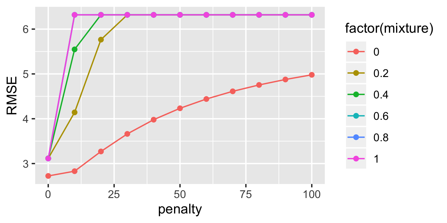

44 / 48

45 / 48

Dr. Lucy D'Agostino McGowan  adapted from Alison Hill's Introduction to ML with the Tidyverse

Putting it all togetherOften we can use a combination of all of these tools together
First split our data
Do cross validation on just the training data to tune the parameters
Use last_fit() with the selected parameters, specifying the split data so that it is evaluated on the left out test sample
46 / 48

Dr. Lucy D'Agostino McGowan  adapted from Alison Hill's Introduction to ML with the Tidyverse

Putting it all togetherauto_split <- initial_split(Auto, prop = 0.5)
auto_train <- training(auto_split)
auto_cv <- vfold_cv(auto_train, v = 5)
rec <- recipe(mpg ~ horsepower + displacement + weight, data = auto_train) %>%
  step_scale(all_predictors())
tuning <- tune_grid(penalty_spec,
                     rec,
                     grid = grid,
                     resamples = auto_cv)
tuning %>%
  collect_metrics() %>%
  filter(.metric == "rmse") %>%
  arrange(mean)

## # A tibble: 66 x 7
##    penalty mixture .metric .estimator  mean     n std_err
##      <dbl>   <dbl> <chr>   <chr>      <dbl> <int>   <dbl>
##  1       0     1   rmse    standard    4.15     5   0.267
##  2       0     0.8 rmse    standard    4.15     5   0.267
##  3       0     0.6 rmse    standard    4.15     5   0.266
##  4       0     0.4 rmse    standard    4.15     5   0.266
##  5       0     0.2 rmse    standard    4.15     5   0.266
##  6       0     0   rmse    standard    4.17     5   0.276
##  7      10     0   rmse    standard    4.60     5   0.428
##  8      20     0   rmse    standard    5.11     5   0.476
##  9      10     0.2 rmse    standard    5.22     5   0.490
## 10      30     0   rmse    standard    5.50     5   0.490
## # … with 56 more rows
47 / 48

Dr. Lucy D'Agostino McGowan  adapted from Alison Hill's Introduction to ML with the Tidyverse

Putting it all togetherfinal_spec <- linear_reg(penalty = 0, mixture = 0) %>%
  set_engine("glmnet")
fit <- last_fit(final_spec,
                rec,
                split = auto_split)
fit %>%
  collect_metrics()

## # A tibble: 2 x 3
##   .metric .estimator .estimate
##   <chr>   <chr>          <dbl>
## 1 rmse    standard       4.43 
## 2 rsq     standard       0.711
48 / 48

↑, ←, Pg Up, k	Go to previous slide
↓, →, Pg Dn, Space, j	Go to next slide
Home	Go to first slide
End	Go to last slide
Number + Return	Go to specific slide
b / m / f	Toggle blackout / mirrored / fullscreen mode
c	Clone slideshow
p	Toggle presenter mode
t	Restart the presentation timer
?, h	Toggle this help

tidymodels

Dr. D’Agostino McGowan

tidymodels

tidymodels

Step 1: Specify the model

Step 1: Specify the model

Specify the model

Specify the model

Specify the model

Specify the model

Specify the model

Specify Model

Fit the data

Fit Model

Get predictions

Get predictions

Get predictions

Get predictions

Get predictions

Get predictions

Get predictions

Calculate the error

Calculate the error

Validation set approach

Validation set approach

Validation set approach

Validation Set

A faster way!

What about cross validation?

What about cross validation?

What about cross validation?

What about cross validation?

What about cross validation?

What about cross validation?

K-fold cross validation

What if we wanted to do some preprocessing

What if we wanted to do some preprocessing

What if we wanted to do some preprocessing

What if we wanted to do some preprocessing

What if we wanted to do some preprocessing

What if we wanted to do some preprocessing

What if we wanted to do some preprocessing

What if we wanted to do some preprocessing

Where do we plug in this recipe?

Where do we plug in this recipe?

What if we want to predict mpg with more variables

What if we want to predict mpg with more variables

What if we want to predict mpg with more variables

Putting it together

Ridge, Lasso, and Elastic net

Ridge, Lasso, and Elastic net

Ridge, Lasso, and Elastic net

Ridge, Lasso, and Elastic net

Ridge, Lasso, and Elastic net

Ridge, Lasso, and Elastic net

Ridge, Lasso, and Elastic net

Lasso specification

Ridge, Lasso, and Elastic net

Ridge, Lasso, and Elastic net

Ridge, Lasso, and Elastic net

Okay, but we wanted to look at 3 different models!

Okay, but we wanted to look at 3 different models!

tune 🎶

tune 🎶

tune 🎶

Subset results

Subset results

Putting it all together

Putting it all together

Putting it all together

tidymodels

Help

`tidymodels`

`Specify Model`

`Fit Model`

`Get predictions`

`Validation Set`

`K-fold cross validation`

`Lasso specification`

`tidymodels`