class: center, middle, inverse, title-slide # Non-linearity ### Dr. D’Agostino McGowan --- layout: true <div class="my-footer"> <span> Dr. Lucy D'Agostino McGowan <i>adapted from slides by Hastie & Tibshirani</i> </span> </div> --- ## Non-linear relationships .question[ What have we used so far to deal with non-linear relationships? ] -- * Hint: What did you use in Lab 03? -- * Polynomials! --- ## Polynomials `$$y_i = \beta_0 + \beta_1x_i + \beta_2x_i^2+\beta_3x_i^3 \dots + \beta_dx_i^d+\epsilon_i$$` <!-- --> -- * This is data from the Columbia World Fertility Survey (1975-76) to examine household compositions -- * Fit here with a 4th degree polynomial --- ## How is it done? * New variables are created ( `\(X_1 = X\)`, `\(X_2 = X^2\)`, `\(X_3 = X^3\)`, etc) and treated as multiple linear regression -- * We are _not_ interested in the individual coefficients, we are interested in how a _specific_ `\(x\)` value behaves `$$\hat{f}(x_0) = \hat\beta_0 + \hat\beta_1x_0 + \hat\beta_2x_0^2 + \hat\beta_3x_0^3 + \hat\beta_4x_0^4$$` -- * _or more often a change between two values_, `\(a\)` and `\(b\)` `$$\hat{f}(b) -\hat{f}(a) = \hat\beta_1b + \hat\beta_2b^2 + \hat\beta_3b^3 + \hat\beta_4b^4 - \hat\beta_1a - \hat\beta_2a^2 - \hat\beta_3a^3 -\hat\beta_4a^4$$` -- `$$\hat{f}(b) -\hat{f}(a) =\hat\beta_1(b-a) + \hat\beta_2(b^2-a^2)+\hat\beta_3(b^3-a^3)+\hat\beta_4(b^4-a^4)$$` --- ## Polynomial Regression `$$\hat{f}(b) -\hat{f}(a) =\hat\beta_1(b-a) + \hat\beta_2(b^2-a^2)+\hat\beta_3(b^3-a^3)+\hat\beta_4(b^4-a^4)$$` .question[ How do you pick `\(a\)` and `\(b\)`? ] -- * If given no other information, a sensible choice may be the 25th and 75th percentiles of `\(x\)` --- ## Polynomial Regression <!-- --> --- class: inverse <div class="countdown" id="timer_5e84a3b9" style="right:0;bottom:0;" data-warnwhen="0"> <code class="countdown-time"><span class="countdown-digits minutes">03</span><span class="countdown-digits colon">:</span><span class="countdown-digits seconds">00</span></code> </div> ## <i class="fas fa-laptop"></i> `Polynomial Regression` `$$pop = \beta_0 + \beta_1age + \beta_2age^2 + \beta_3age^3 +\beta_4age^4+ \epsilon$$` Using the information below, write out the equation to predicted change in population from a change in age from the 25th percentile (24.5) to a 75th percentile (73.5). |term | estimate| std.error| statistic| p.value| |:-----------|---------:|---------:|---------:|-------:| |(Intercept) | 1672.0854| 64.5606| 25.8995| 0.0000| |age | -10.6429| 9.2268| -1.1535| 0.2516| |I(age^2) | -1.1427| 0.3857| -2.9627| 0.0039| |I(age^3) | 0.0216| 0.0059| 3.6498| 0.0004| |I(age^4) | -0.0001| 0.0000| -3.6540| 0.0004| --- ## Choosing `\(d\)` `$$y_i = \beta_0 + \beta_1x_i + \beta_2x_i^2+\beta_3x_i^3 \dots + \beta_dx_i^d+\epsilon_i$$` ## Either: * Pre-specify `\(d\)` (before looking 👀 at your data!) * Use cross-validation to pick `\(d\)` -- .question[ Why? ] --- ## Polynomial Regression * polynomials have notoriously bad tail behavior (so they can be bad for extrapolation) -- .question[ What does this mean? ] --- ## Step functions * Another way to create a transformation is to cut the variable into distinct regions `$$C_1(X) = I(X < 35), C_2(X) = I(35\leq X<65), C_3(X) = I(X \geq 65)$$` <!-- --> --- ## Step functions * Create dummy variables for each group -- * Include each of these variables in multiple regression -- * The choice of cutpoints or **knots** can be problematic (and make a big difference!) --- ## Step functions `$$C_1(X) = I(X < 35), C_2(X) = I(35\leq X<65), C_3(X) = I(X \geq 65)$$` <!-- --> -- `$$C_1(X) = I(X < 15), C_2(X) = I(15\leq X<65), C_3(X) = I(X \geq 65)$$` <!-- --> --- ## Piecewise polynomials * Instead of a single polynomial in `\(X\)` over it's whole domain, we can use different polynomials in regions defined by knots `$$y_i = \begin{cases}\beta_{01}+\beta_{11}x_i + \beta_{21}x^2_i+\beta_{31}x^3_i+\epsilon_i& \textrm{if } x_i < c\\ \beta_{02}+\beta_{12}x_i + \beta_{22}x_i^2 + \beta_{32}x_{i}^3+\epsilon_i&\textrm{if }x_i\geq c\end{cases}$$` -- .question[ What could go wrong here? ] -- * It would be nice to have constraints (like continuity!) -- * Insert **splines!** ---  --- ## Linear Splines _A linear spline with knots at `\(\xi_k\)`, `\(k = 1,\dots, K\)` is a piecewise linear polynomial continuous at each knot_ -- `$$y_i = \beta_0 + \beta_1b_1(x_i)+\beta_2b_2(x_i)+\dots+\beta_{K+1}b_{K+1}(x_i)+\epsilon_i$$` -- * `\(b_k\)` are **basis functions** `$$\begin{align}b_1(x_i)&=x_i\\ b_{k+1}(x_i)&=(x_i-\xi_k)_+,k=1,\dots,K\end{align}$$` -- Here `\(()_+\)` means the **positive part** `$$(x_i-\xi_k)_+=\begin{cases}x_i-\xi_k & \textrm{if } x_i>\xi_k\\0&\textrm{otherwise}\end{cases}$$` ---  --- ## Cubic Splines _A cubic spliens with knots at `\(\xi_i, k = 1, \dots, K\)` is a piecewise cubic polynomial with continuous derivatives up to order 2 at each knot._ -- Again we can represent this model with truncated power functions `$$y_i = \beta_0 + \beta_1b_1(x_i)+\beta_2b_2(x_i)+\dots+\beta_{K+3}b_{K+3}(x_i) + \epsilon_i$$` `$$\begin{align}b_1(x_i)&=x_i\\b_2(x_i)&=x_i^2\\b_3(x_i)&=x_i^3\\b_{k+3}(x_i)&=(x_i-\xi_k)^3_+, k = 1,\dots,K\end{align}$$` -- where `$$(x_i-\xi_k)^{3}_+=\begin{cases}(x_i-\xi_k)^3&\textrm{if }x_i>\xi_k\\0&\textrm{otherwise}\end{cases}$$` ---  --- ## Natural cubic splines _A natural cubic spline extrapolates linearly beyond the boundary knots_ -- * This adds 4 extra constraints and allows us to put **more** internal knots for the same degrees of freedom as a regular cubic spline <img src="img/13/natural.png" height=400></img> --- ## Knot placement * One strategy is to decide `\(K\)` (the number of knots) in advance and then place them at appropriate quantiles of the observed `\(X\)` -- * A cubic spline with `\(K\)` knots has `\(K+4\)` parameters (or degrees of freedom!) -- * A natural spline with `\(K\)` knots has `\(K\)` degrees of freedom --- ## Knot placement * Here is a comparision of a degree-14 polynomial and natural cubic spline (both have 15 degrees of freedom) 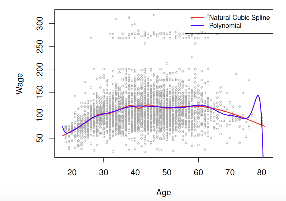 ---